2D SBP
After reading the Global View and Global Tensor, you may have learned about the basic concepts of SBP and SBP Signature, and can get started with related tasks. In fact, both these two documents refers to 1D SBP.
Since you have known about 1D SBP, this document introduces 2D SBP, which can more flexibly deal with more complex distributed training scenarios.
2D Devices Array
We are already familiar with the placement configuration of 1D SBP. In the scenario of 1D SBP, configure the cluster through the oneflow.placement interface. For example, use the 0~3 GPU graphics in the cluster:
>>> placement1 = flow.placement("cuda", ranks=[0, 1, 2, 3])
The above "cuda" specifies the device type, and ranks=[0, 1, 2, 3] specifies the computing devices in the cluster. In fact, ranks can be not only a one-dimensional int list, but also a multi-dimensional int array:
>>> placement2 = flow.placement("cuda", ranks=[[0, 1], [2, 3]])
When ranks is in the form of a one-dimensional list like ranks=[0, 1, 2, 3], all devices in the cluster form a 1D device vector, which is where the 1D SBP name comes from.
When ranks is in the form of a multi-dimensional array, the devices in the cluster are grouped into a multi-dimensional array of devices. ranks=[[0, 1], [2, 3]] means that the four computing devices in the cluster are divided into a \(2 \times 2\) device array.
2D SBP
When constructing a Global Tensor, we need to specify both placement and SBP. When the cluster in placement is a 2-dimensional device array, SBP must also correspond to it, being a tuple with a length of 2. The 0th and 1st elements in this tuple respectively describes the distribution of Global Tensor in the 0th and 1st dimensions of the device array.
For example, The following code configures a \(2 \times 2\) device array, and sets the 2D SBP to (broadcast, split(0)).
>>> a = flow.Tensor([[1,2],[3,4]])
>>> placement = flow.placement("cuda", ranks=[[0, 1], [2, 3]])
>>> sbp = (flow.sbp.broadcast, flow.sbp.split(0))
>>> a_to_global = a.to_global(placement=placement, sbp=sbp)
It means that logically the data, over the entire device array, is broadcast in the 0th dimension ("viewed vertically"); split(0) in the 1st dimension ("viewed across").
See the following figure:
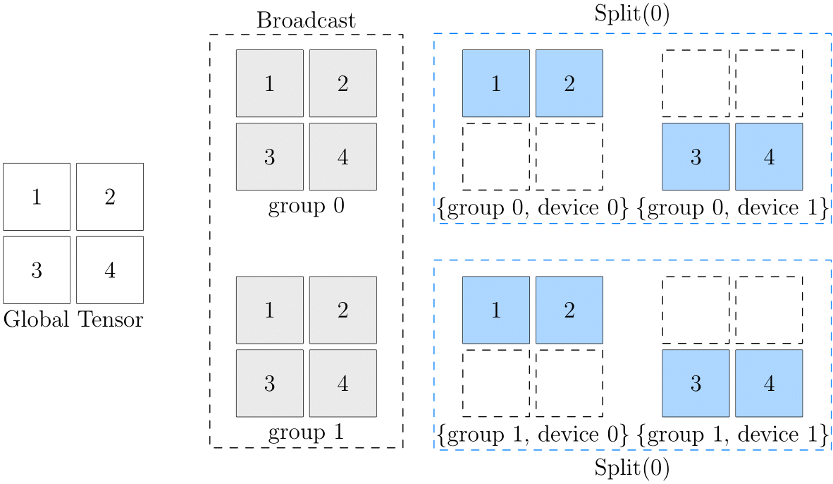
In the above figure, the left side is the global data, and the right side is the data of each device on the device array. As you can see, from the perspective of the 0th dimension, they are all in broadcast relations:
- The data in (group0, device0) and (group1, device0) are consistent, and they are in
broadcastrelations to each other - The data in (group0, device1) and (group1, device1) are consistent, and they are in
broadcastrelations to each other
From the perspective of the 1st dimension, they are all in split(0) relations:
- (group0, device0) and (group0, device1) are in
split(0)relations to each other - (group1, device0) and (group1, device1) are in
split(0)relations to each other
It may be difficult to directly understand the correspondence between logical data and physical data in the final device array. When thinking about 2D SBP, you can imagine an intermediate state (gray part in the above figure) there. Take (broadcast, split(0)) as an example:
- First, the original logical tensor is broadcast to 2 groups through
broadcast, and the intermediate state is obtained - On the basis of the intermediate state,
split(0)is continued to be done on the groups to get the status of each physical tensor in the final device array
2D SBP Signature
1D SBP has the concept of SBP signature, similarly, the operator also has 2D SBP signature. Based on mastering the concept of 1D SBP and its signature concept, 2D SBP signature is very simple and you only need to follow one principle:
- Independently derive in the respective dimensions
Let's take matrix multiplication as an example. First, let's review the case of 1D SBP. Suppose that \(x \times w = y\) can have the following SBP Signature:
and
Now, suppose we set the 2D SBP for \(x\) to \((broadcast, split(0))\) and set the 2D SBP for \(w\) to \((split(1), broadcast)\), then in the context of the 2D SBP, operate \(x \times w = y\) to obtain the SBP attribute for \(y\) is \((split(1), split(0))\).
That is to say, the following 2D SBPs constitute the 2D SBP Signature of matrix multiplication:
An Example of Using 2D SBP
In this section, we are going to use a simple example to demonstrate how to conduct distributed training using 2D SBP. Same as the example above, assume that there is a \(2 \times 2\) device array. Given that readers may not have multiple GPU devices at present, we will use CPU to simulate the case of \(2 \times 2\) device array. We adopt the parallelism strategy (broadcast, split(0)) in the above figure to the input tensor.
First of all, import the dependencies:
import oneflow as flow
import oneflow.nn as nn
Then, define the placement and SBP that will be used:
PLACEMENT = flow.placement("cpu", [[0, 1], [2, 3]])
BROADCAST = (flow.sbp.broadcast, flow.sbp.broadcast)
BS0 = (flow.sbp.broadcast, flow.sbp.split(0))
ranks of PLACEMENT is a two-dimensional list, which represents that the devices in the cluster are divided into a device array of \(2 \times 2\). As mentioned earlier, the SBP needs to correspond to it and be specified as a tuple with a length of 2. BROADCAST means broadcasting on both the 0th and 1st dimensions of the device array, and the meaning of BS0 is the same as the description above.
Assume that we have the following model:
model = nn.Sequential(nn.Linear(8, 4),
                      nn.ReLU(),
                      nn.Linear(4, 2))
Broadcast the model on the cluster:
model = model.to_global(placement=PLACEMENT, sbp=BROADCAST)
And construct the data and carry out forward inference:
x = flow.randn(1, 2, 8)
global_x = x.to_global(placement=PLACEMENT, sbp=BS0)
pred = model(global_x)
(1, 2, 8), and obtain the corresponding global tensor through Tensor.to_global method. Finally, input it to the model for inference.
After obtaining the local tensor on current physical device through Tensor.to_local method, we can output its shape and value to verify whether the data has been processed correctly:
local_x = global_x.to_local()
print(f'{local_x.device}, {local_x.shape}, \n{local_x}')
cpu:2, oneflow.Size([1, 2, 8]),
tensor([[[ 0.6068,  0.1986, -0.6363, -0.5572, -0.2388,  1.1607, -0.7186,  1.2161],
         [-0.1632, -1.5293, -0.6637, -1.0219,  0.1464,  1.1574, -0.0811, -1.6568]]], dtype=oneflow.float32)
cpu:3, oneflow.Size([1, 2, 8]),
tensor([[[-0.7676,  0.4519, -0.8810,  0.5648,  1.5428,  0.5752,  0.2466, -0.7708],
         [-1.2131,  1.4590,  0.2749,  0.8824, -0.8286,  0.9989,  0.5599, -0.5099]]], dtype=oneflow.float32)
cpu:1, oneflow.Size([1, 2, 8]),
tensor([[[-0.7676,  0.4519, -0.8810,  0.5648,  1.5428,  0.5752,  0.2466, -0.7708],
         [-1.2131,  1.4590,  0.2749,  0.8824, -0.8286,  0.9989,  0.5599, -0.5099]]], dtype=oneflow.float32)
cpu:0, oneflow.Size([1, 2, 8]),
tensor([[[ 0.6068,  0.1986, -0.6363, -0.5572, -0.2388,  1.1607, -0.7186,  1.2161],
         [-0.1632, -1.5293, -0.6637, -1.0219,  0.1464,  1.1574, -0.0811, -1.6568]]], dtype=oneflow.float32)
It should be noted that we cannot directly use python xxx.py to run the above code, but need to launch through oneflow.distributed.launch. This module can easily start distributed training. Execute the following command in the terminal (It is assumed that the above code has been saved to a file named "2d_sbp.py" in the current directory)
python3 -m oneflow.distributed.launch --nproc_per_node=4 2d_sbp.py
nproc_per_node is assigned as 4 to create 4 processes, simulating a total of 4 GPUs. For detailed usage of this module, please read: DISTRIBUTED TRAINING LAUNCHER.
The complete code is as follows:
Code
PLACEMENT = flow.placement("cpu", [[0, 1], [2, 3]])
BROADCAST = (flow.sbp.broadcast, flow.sbp.broadcast)
BS0 = (flow.sbp.broadcast, flow.sbp.split(0))

model = nn.Sequential(nn.Linear(8, 4),
                      nn.ReLU(),
                      nn.Linear(4, 2))
model = model.to_global(placement=PLACEMENT, sbp=BROADCAST)

x = flow.randn(1, 2, 8)
global_x = x.to_global(placement=PLACEMENT, sbp=BS0)
pred = model(global_x)

local_x = global_x.to_local()
print(f'{local_x.device}, {local_x.shape}, \n{local_x}')