STATIC GRAPH INTERFACE: NN.GRAPH

At present, there are two ways to run models in deep learning framework, Dynamic Graph and Static Graph, which are also called Eager Mode and Graph Mode in OneFlow.

There are pros and cons to both approaches, and OneFlow offers support for both, with the Eager Mode by default. If you are reading the tutorials for this basic topic in order, then all the code you have encountered so far is in Eager Mode.

In general, dynamic graphs are easier to use and static graphs have better performance. OneFlow offers nn.Graph, so that users can use the eager-like programming style to build static graphs and train the models.

Eager Mode in OneFlow

OneFlow runs in Eager Mode by default.

The following script uses data set CIFAR10 to train model mobilenet_v2.

Code

import oneflow as flow
import oneflow.nn as nn
import flowvision
import flowvision.transforms as transforms

BATCH_SIZE=64
EPOCH_NUM = 1

DEVICE = "cuda" if flow.cuda.is_available() else "cpu"
print("Using {} device".format(DEVICE))

training_data = flowvision.datasets.CIFAR10(
    root="data",
    train=True,
    transform=transforms.ToTensor(),
    download=True,
    source_url="https://oneflow-public.oss-cn-beijing.aliyuncs.com/datasets/cifar/cifar-10-python.tar.gz",
)

train_dataloader = flow.utils.data.DataLoader(
    training_data, BATCH_SIZE, shuffle=True
)

model = flowvision.models.mobilenet_v2().to(DEVICE)
model.classifer = nn.Sequential(nn.Dropout(0.2), nn.Linear(model.last_channel, 10))
model.train()

loss_fn = nn.CrossEntropyLoss().to(DEVICE)
optimizer = flow.optim.SGD(model.parameters(), lr=1e-3)


for t in range(EPOCH_NUM):
    print(f"Epoch {t+1}\n-------------------------------")
    size = len(train_dataloader.dataset)
    for batch, (x, y) in enumerate(train_dataloader):
        x = x.to(DEVICE)
        y = y.to(DEVICE)

        # Compute prediction error
        pred = model(x)
        loss = loss_fn(pred, y)

        # Backpropagation
        optimizer.zero_grad()
        loss.backward()
        optimizer.step()

        current = batch * BATCH_SIZE
        if batch % 5 == 0:
            print(f"loss: {loss:>7f}  [{current:>5d}/{size:>5d}]")

Out:

loss: 6.921304  [    0/50000]
loss: 6.824391  [  320/50000]
loss: 6.688272  [  640/50000]
loss: 6.644351  [  960/50000]
...

Graph Mode in OneFlow

Customize a Graph

OneFlow provide the base class nn.Graph, which can be inherited to create a customized Graph class.

import oneflow as flow
import oneflow.nn as nn

class ModuleMyLinear(nn.Module):
    def __init__(self, in_features, out_features):
        super().__init__()
        self.weight = nn.Parameter(flow.randn(in_features, out_features))
        self.bias = nn.Parameter(flow.randn(out_features))

    def forward(self, input):
        return flow.matmul(input, self.weight) + self.bias

linear_model = ModuleMyLinear(4, 3)

class GraphMyLinear(nn.Graph):
  def __init__(self):
    super().__init__()
    self.model = linear_model

  def build(self, input):
    return self.model(input)

The simple example above contains the important steps needed to customize a Graph:

• Inherits nn.Graph.
• Call super().__init__() at the begining of __init__ method to get OneFlow to do the necessary initialization for the Graph.
• In __init__, reuse the nn.Module object in Eager mode (self.model = model)
• Describes the computational process in build method.

You can then instantiate and call the Graph:

graph_mylinear = GraphMyLinear()
input = flow.randn(1, 4)
out = graph_mylinear(input)
print(out)

Out:

tensor([[-0.3298, -3.7907,  0.1661]], dtype=oneflow.float32)

Note that Graph is similar to Module in that the object itself is callable and it is not recommended to explicitly call the build method. Graph can directly reuse a defined Module. Users can refer the content in Build Network to build a neural network. Then, set Module as a member of Graph in __init__ of Graph.

For example, use the linear_model above as the network structure:

class ModelGraph(flow.nn.Graph):
    def __init__(self):
        super().__init__()
        self.model = linear_model

    def build(self, x, y):
        y_pred = self.model(x)
        return loss

model_graph = ModelGraph()

The major difference between Module and Graph is that Graph uses build method rather than forward method to describe the computation process, because the build method can contain not only forward computation, but also setting loss, optimizer, etc. You will see an example of using Graph for training later.

Inference in Graph Mode

The following example for inference in Graph Mode directly using the model, which we have already trained in Eager Mode at the beginning of this article.

class GraphMobileNetV2(flow.nn.Graph):
    def __init__(self):
        super().__init__()
        self.model = model

    def build(self, x):
        return self.model(x)


graph_mobile_net_v2 = GraphMobileNetV2()

x, _ = next(iter(train_dataloader))
x = x.to(DEVICE)
y_pred = graph_mobile_net_v2(x)

Training in Graph Mode

The Graph can be used for training. Click on the "Code" below to see the detailed code.

Code

import oneflow as flow
import oneflow.nn as nn
import flowvision
import flowvision.transforms as transforms

BATCH_SIZE=64
EPOCH_NUM = 1

DEVICE = "cuda" if flow.cuda.is_available() else "cpu"
print("Using {} device".format(DEVICE))

training_data = flowvision.datasets.CIFAR10(
    root="data",
    train=True,
    transform=transforms.ToTensor(),
    download=True,
)

train_dataloader = flow.utils.data.DataLoader(
    training_data, BATCH_SIZE, shuffle=True, drop_last=True
)

model = flowvision.models.mobilenet_v2().to(DEVICE)
model.classifer = nn.Sequential(nn.Dropout(0.2), nn.Linear(model.last_channel, 10))
model.train()

loss_fn = nn.CrossEntropyLoss().to(DEVICE)
optimizer = flow.optim.SGD(model.parameters(), lr=1e-3)

class GraphMobileNetV2(flow.nn.Graph):
    def __init__(self):
        super().__init__()
        self.model = model
        self.loss_fn = loss_fn
        self.add_optimizer(optimizer)

    def build(self, x, y):
        y_pred = self.model(x)
        loss = self.loss_fn(y_pred, y)
        loss.backward()
        return loss


graph_mobile_net_v2 = GraphMobileNetV2()
# graph_mobile_net_v2.debug()

for t in range(EPOCH_NUM):
    print(f"Epoch {t+1}\n-------------------------------")
    size = len(train_dataloader.dataset)
    for batch, (x, y) in enumerate(train_dataloader):
        x = x.to(DEVICE)
        y = y.to(DEVICE)
        loss = graph_mobile_net_v2(x, y)
        current = batch * BATCH_SIZE
        if batch % 5 == 0:
            print(f"loss: {loss:>7f}  [{current:>5d}/{size:>5d}]")

Comparing to inference, there are only a few things that are unique to training:

# Optimizer
optimizer = flow.optim.SGD(model.parameters(), lr=1e-3) # (1)

# The MobileNetV2 Graph
class GraphMobileNetV2(flow.nn.Graph):
    def __init__(self):
        # ...
        self.add_optimizer(optimizer) # (2)

    def build(self, x, y):
        # ...
        loss.backward() # (3)
        # ...

1. Constructing the optimizer object, which is same to the training in Eager Mode introduced in Backpropagation and Optimizer.
2. Call self.add_optimizer in Graph's __init__ method to add the optimizer object constructed in the previous step to the Graph.
3. Call backward in Graph's build to trigger back propagation.

Debugging in Graph Mode

There are two ways to show the debug information of the Graph at present. Firstly you can call print to print the Graph object, and show information about it.

print(graph_mobile_net_v2)

The output is slightly different depending on whether the Graph object has been called:

If you use print before the Graph object is called, the output is information about the network structure.

The output for print used before graph_mobile_net_v2 is called is like this:

(GRAPH:GraphMobileNetV2_0:GraphMobileNetV2): (
  (CONFIG:config:GraphConfig(training=True, ))
  (MODULE:model:MobileNetV2()): (
    (MODULE:model.features:Sequential()): (
      (MODULE:model.features.0:ConvBNActivation()): (
        (MODULE:model.features.0.0:Conv2d(3, 32, kernel_size=(3, 3), stride=(2, 2), padding=(1, 1), bias=False)): (
          (PARAMETER:model.features.0.0.weight:tensor(..., device='cuda:0', size=(32, 3, 3, 3), dtype=oneflow.float32,
                 requires_grad=True)): ()
        )
    ...
    (MODULE:model.classifer:Sequential()): (
      (MODULE:model.classifer.0:Dropout(p=0.2, inplace=False)): ()
      (MODULE:model.classifer.1:Linear(in_features=1280, out_features=10, bias=True)): (
        (PARAMETER:model.classifer.1.weight:tensor(..., size=(10, 1280), dtype=oneflow.float32, requires_grad=True)): ()
        (PARAMETER:model.classifer.1.bias:tensor(..., size=(10,), dtype=oneflow.float32, requires_grad=True)): ()
      )
    )
  )
  (MODULE:loss_fn:CrossEntropyLoss()): ()
)

In the above debug information, it means that based on Sequential model, the network customizes structures such as ConvBNActivation ( Corresponds to the MBConv module ), convolutional layer( including detailed parameter information such as channel, kernel_size and stride ), Dropout and fully connected layer.

If you use print after the Graph object is called, in addition to the structure of the network, it will print inputs and outputs of the tensors, the output on the console is like this:

(GRAPH:GraphMobileNetV2_0:GraphMobileNetV2): (
  (CONFIG:config:GraphConfig(training=True, ))
  (INPUT:_GraphMobileNetV2_0-input_0:tensor(..., device='cuda:0', size=(64, 3, 32, 32), dtype=oneflow.float32))
  (INPUT:_GraphMobileNetV2_0-input_1:tensor(..., device='cuda:0', size=(64,), dtype=oneflow.int64))
  (MODULE:model:MobileNetV2()): (
    (INPUT:_model-input_0:tensor(..., device='cuda:0', is_lazy='True', size=(64, 3, 32, 32),
           dtype=oneflow.float32))
    (MODULE:model.features:Sequential()): (
      (INPUT:_model.features-input_0:tensor(..., device='cuda:0', is_lazy='True', size=(64, 3, 32, 32),
             dtype=oneflow.float32))
      (MODULE:model.features.0:ConvBNActivation()): (
        (INPUT:_model.features.0-input_0:tensor(..., device='cuda:0', is_lazy='True', size=(64, 3, 32, 32),
               dtype=oneflow.float32))
        (MODULE:model.features.0.0:Conv2d(3, 32, kernel_size=(3, 3), stride=(2, 2), padding=(1, 1), bias=False)): (
          (INPUT:_model.features.0.0-input_0:tensor(..., device='cuda:0', is_lazy='True', size=(64, 3, 32, 32),
                 dtype=oneflow.float32))
          (PARAMETER:model.features.0.0.weight:tensor(..., device='cuda:0', size=(32, 3, 3, 3), dtype=oneflow.float32,
                 requires_grad=True)): ()
          (OUTPUT:_model.features.0.0-output_0:tensor(..., device='cuda:0', is_lazy='True', size=(64, 32, 16, 16),
                 dtype=oneflow.float32))
        )
    ...

The second way is that by calling the debug method of Graph objects, Graph’s debug mode is turned on.

graph_mobile_net_v2.debug(v_level=1) # The defalut of v_level is 0.

which can also be written in a simplified way:

graph_mobile_net_v2.debug(1)

OneFlow prints debug information when it compiles the computation graph. If the graph_mobile_net_v2.debug() is removed from the example code above, the output on the console is like this:

(GRAPH:GraphMobileNetV2_0:GraphMobileNetV2) end building graph.
(GRAPH:GraphMobileNetV2_0:GraphMobileNetV2) start compiling plan and init graph runtime.
(GRAPH:GraphMobileNetV2_0:GraphMobileNetV2) end compiling plan and init graph rumtime.

The advantage of using debug is that the debug information is composed and printed at the same time, which makes it easy to find the problem if there is any error in the graph building process.

Use v_level to choose verbose debug info level, default level is 0, max level is 3.

• v_level=0 will only print basic information of warning and graph building stages, like graph building time.
• v_level=1 will additionally print graph build info of each nn.Module, the specific content is described in the table below.
• v_level=2 will additionally print graph build info of each operation in graph building stages, including name, input, device, SBP information, etc.
• v_level=3 will additionally print more detailed info of each operation, like information about the location of the code, which is convenient for locating problems in file.

In addition, in order for developers to have a clearer understanding of the types under the Graph object, the following is an analysis of the output of debug, which basically includes seven categories of tags: GRAPH, CONFIG, MODULE, PARAMETER, BUFFER, INPUT and OUTPUT.

Name	Info	Example
GRAPH	User-defined Graph information, followed by type: name: construction method.	(GRAPH:GraphMobileNetV2_0:GraphMobileNetV2)
CONFIG	Graph configuration information. training=True indicates that the Graph is in training mode, and if in the evaluation mode, it corresponds to training=False.	(CONFIG:config:GraphConfig(training=True, )
MODULE	Corresponding to nn.Module , MODULE can be under the Graph tag, and there is also a hierarchical relationship between multiple modules.	(MODULE:model:MobileNetV2()), and MobileNetV2 reuses the Module class name in Eager mode for users.
PARAMETER	Shows the clearer information of weight and bias. In addition, when building the graph, the data content of the tensor is less important, so it is more important for building network to only display the meta information of the tensor.	(PARAMETER:model.features.0.1.weight:tensor(..., device='cuda:0', size=(32,), dtype=oneflow.float32, requires_grad=True))
BUFFER	Statistical characteristics and other content generated during training, such as running_mean and running_var.	(BUFFER:model.features.0.1.running_mean:tensor(..., device='cuda:0', size=(32,), dtype=oneflow.float32))
INPUT & OUPTUT	Tensor information representing input and output.	(INPUT:_model_input.0.0_2:tensor(..., device='cuda:0', is_lazy='True', size=(16, 3, 32, 32), dtype=oneflow.float32))

In addition to the methods described above, getting the parameters of the gradient during the training process, accessing to the learning rate and other functions are also under development and will come up soon.

Save and Load Graph Models

When training Graph model, it is often necessary to save the parameters of the model that has been trained for a period of time and other states such as optimizer parameters, so as to facilitate the resume of training after interruption.

Graph model objects have state_dict and load_state_dict interfaces that similar to Module. We can save and load graph models with save and load. This is similar to Eagar module introduced in Model Save and Load. A little different from Eager mode is that when calling Graph's state_dict during training, in addition to the parameters of each layer of the internal Module, other states such as training iteration steps and optimizer parameters will also be obtained, so as to resume training later.

For example, we hope to save the latest state after each epoch while training graph_mobile_net_v2 above, we need to add the following code:

Assume that we want to save into "GraphMobileNetV2" under current directory:

CHECKPOINT_SAVE_DIR = "./GraphMobileNetV2"

Insert the following code at the completion of each epoch:

import shutil
shutil.rmtree(CHECKPOINT_SAVE_DIR, ignore_errors=True)  # Clear previous state
flow.save(graph_mobile_net_v2.state_dict(), CHECKPOINT_SAVE_DIR)

Note

Don't save in the following way. Because Graph will process members when it is initialized, and graph_mobile_net_v2.model is actually no longer a Module type:

flow.save(graph_mobile_net_v2.model.state_dict(), CHECKPOINT_SAVE_DIR)  # it will report an error

When we need to restore the previously saved state:

state_dict = flow.load(CHECKPOINT_SAVE_DIR)
graph_mobile_net_v2.load_state_dict(state_dict)

Graph and Deployment

nn.Graph supports saving model parameters and computation graph at the same time, which can easily support model deployment.

If there is a need for model deployment, the Graph object should be exported to the format required for deployment through the oneflow.save interface:

MODEL_SAVE_DIR="./mobile_net_v2_model"
import os
if not os.path.exists(MODEL_SAVE_DIR):
    os.makedirs(MODEL_SAVE_DIR)
flow.save(graph_mobile_net_v2, MODEL_SAVE_DIR)

Note

Note the difference from the previous section. save interface supports saving state_dict and also Graph objects. When the Graph object is saved, the model parameters and computation graph will be saved at the same time to decouple from the model structure definition code.

In this way, both model parameters and computation graph required for deployment will be saved in the ./mobile_net_v2_model directory. For detailed deployment process, refer to Model Deployment.

You must export the model via a Graph object to meet the format requirement for deployment. If it is a model trained in Eager mode (i.e. nn.Module object), you need to use Graph to encapsulate the Module and then export it.

Next, we take the neural_style_transfer as an example in the flowvision repository to show how to encapsulate and export the nn.Module model.

import oneflow as flow
import oneflow.nn as nn
from flowvision.models.neural_style_transfer.stylenet import neural_style_transfer


class MyGraph(nn.Graph):
    def __init__(self, model):
        super().__init__()
        self.model = model

    def build(self, *input):
        return self.model(*input)


if __name__ == "__main__":
    fake_image = flow.ones((1, 3, 256, 256))
    model = neural_style_transfer(pretrained=True, progress=True)
    model.eval()
    graph = MyGraph(model)
    out = graph(fake_image)

    MODEL_SAVE_DIR="./neural_style_transfer_model"
    import os
    if not os.path.exists(MODEL_SAVE_DIR):
        os.makedirs(MODEL_SAVE_DIR)
    flow.save(graph, MODEL_SAVE_DIR)

The above code:

• Defines a MyGraph class, and simply encapsulates the nn.Module object (return self.model(*input)), which is only used to convert nn.Module into a Graph object
• Instantiates the model to get the Graph object（graph = MyGraph(model))
• Calls once the Graph object (out = graph(fake_image)). Its internal mechanism is to use "fake data" to flow through the model (tracing mechanism) to build a computation graph
• Exports the model required for deployment:flow.save(graph, "1/model")

Further Reading: Dynamic Graph vs. Static Graph

User-defined neural networks, are transformed by deep learning frameworks into computation graphs, like the example in Autograd:

def loss(y_pred, y):
    return flow.sum(1/2*(y_pred-y)**2)

x = flow.ones(1, 5)  # the input
w = flow.randn(5, 3, requires_grad=True)
b = flow.randn(1, 3, requires_grad=True)
z = flow.matmul(x, w) + b

y = flow.zeros(1, 3)  # the label
l = loss(z,y)

The corresponding computation graph is:

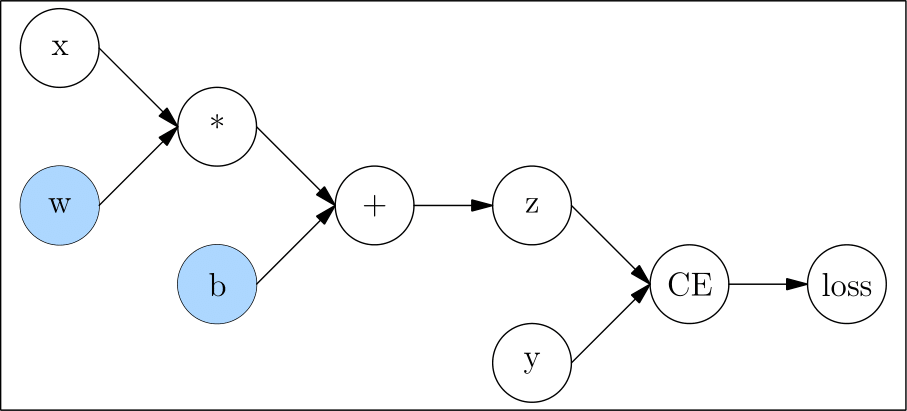
Dynamic Graph

The characteristic of dynamic graph is that it is defined by run.

The code above is run like this (Note: the figure below merges simple statements):

Because the dynamic graph is defined by run, it is very flexible and easy to debug. You can modify the graph structure at any time and get results immediately. However, the deep learning framework can not get the complete graph information(which can be changed at any time and can never be considered as finished), it can not make full global optimization, so its performance is relatively poor.

Static Graph

Unlike a dynamic graph, a static graph defines a complete computation graph. It requires the user to declare all compute nodes before the framework starts running. This can be understood as the framework acting as a compiler between the user code and the computation graph that ultimately runs.

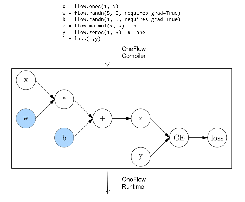
In the case of the OneFlow, the user’s code is first converted to a full computation graph and then run by the OneFlow Runtime module.

Static graph, which get the complete network first, then compile and run, can be optimized in a way that dynamic graph can not, so they have an advantage in performance. It is also easier to deploy across platforms after compiling the computation graph.

However, when the actual computation takes place in a static graph, it is no longer directly related to the user’s code, so debugging the static graph is not convenient.

The two approaches can be summarized as follows:

	Dynamic Graph	Static Graph
Computation Mode	Eager Mode	Graph Mode
Pros	The code is flexible and easy to debug.	Good performance, easy to optimize and deploy.
Cons	Poor performance and portability.	Not easy to debug.

The Eager Mode in OneFlow is aligned with the PyTorch, which allows users familiar with the PyTorch to get their hands on easily with no more effert.

The Graph Mode in OneFlow is based on the object-oriented programming style, which allows developers familiar with eager programming style to benefit from static graph with minimal code changes.

Related Links

Building neural network in OneFlow Eager Mode: Build Network